Balancing Data for Better Predictions: The Power of Oversampling in Machine Learning
In the realm of machine learning, data serves as the lifeblood, but its quality can determine the success or failure of predictive models. One common challenge is dealing with imbalanced datasets, where certain classes are significantly underrepresented compared to others. This imbalance is particularly problematic in fields like fraud detection, disease diagnosis, and anomaly identification.
Understanding the Challenge
When classification algorithms are trained on imbalanced data, they tend to favor the majority class. This bias leads to poor predictive accuracy, as the model overlooks crucial patterns and insights hidden within minority class examples. Real-world applications often require sensitivity to rare but critical events, making traditional modeling approaches impractical.
The Role of Oversampling
Oversampling emerges as a solution to rebalance skewed datasets before model training begins. By increasing the number of instances in the minority class, oversampling ensures that the model learns equally from all classes. This prevents the algorithm from disregarding important yet scarce data points.
Techniques in Action
Common oversampling techniques include:
Random Oversampling: Duplicates minority class instances to match the majority class.
SMOTE (Synthetic Minority Oversampling Technique): Generates synthetic data points by interpolating between existing minority class instances.
ADASYN (Adaptive Synthetic Sampling Approach for Imbalanced Learning):Similar to SMOTE but focuses on regions where minority examples are dense.
Practical Implementation
Python libraries like imbalanced-learn and Scikit-learn offer utilities to implement oversampling techniques. Researchers and data scientists can compare model performances on original versus oversampled datasets to assess improvements in evaluation metrics such as recall, precision, and F1-score for minority classes.
Benefits and Considerations
While oversampling mitigates the pitfalls of imbalanced learning, careful implementation is crucial to avoid overfitting and maintain model generalizability. By restoring balance to the data, machine learning models become more adept at handling critical use cases requiring sensitivity to rare events and outliers.
What is Oversampling?
Oversampling is a data augmentation technique used to rectify class imbalance issues in machine learning. It involves increasing the number of minority class samples either through replication of existing instances or generation of synthetic data points. This process aims to level out the distribution of class frequencies, ensuring more balanced and reliable model training.
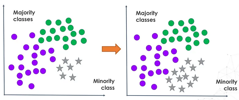
By employing oversampling techniques before model training, underrepresented classes are amplified to ensure learned patterns more accurately represent all categories, rather than favoring dominant ones. This approach enhances various evaluation metrics, particularly crucial for detecting infrequent yet significant events.
Why Do We Need Oversampling?
In imbalanced datasets, accurately classifying minority classes is paramount. The cost of missing these classes (false negatives) outweighs falsely identifying samples (false positives). Traditional machine learning algorithms like logistic regression and random forests optimize for overall accuracy, assuming balanced class distributions. This bias leads models to favor the majority class, missing patterns crucial to sparse but critical classes.
Advantages of Oversampling
By rebalancing datasets through oversampling, misclassification costs are equitably distributed across outcomes. This ensures classifiers can identify underrepresented categories more accurately, reducing costly false negatives.
Oversampling vs. Undersampling
Both techniques aim to balance class distributions, but they approach it differently:
Oversampling increases the minority class by replicating or generating new examples.
Undersampling reduces the majority class to achieve balance.
Undersampling is effective when the majority class has redundant samples or with large datasets, though it risks losing information and biasing models. Conversely, oversampling is beneficial for small datasets with limited minority class samples but may lead to overfitting or unrealistic data synthesis.
Types of Oversampling Approaches
1. Random Oversampling: Duplicates minority class examples randomly to achieve class balance. It efficiently boosts minority observations in small datasets without requiring additional real-world data collection.
Implementing random oversampling can be straightforward using tools like RandomOverSampler from the imbalanced-learn library. This method provides a foundational approach for addressing imbalance, serving as a baseline for comparing more advanced oversampling techniques.
from imblearn.over_sampling import RandomOverSampler
from imblearn.pipeline import make_pipeline

X, y = create_dataset(n_samples=100, weights=(0.05, 0.25, 0.7))

fig, axs = plt.subplots(nrows=1, ncols=2, figsize=(15, 7))

clf.fit(X, y)
plot_decision_function(X, y, clf, axs[0], title="Without resampling")

sampler = RandomOverSampler(random_state=0)
model = make_pipeline(sampler, clf).fit(X, y)
plot_decision_function(X, y, model, axs[1],
                       f"Using {model[0].__class__.__name__}")

fig.suptitle(f"Decision function of {clf.__class__.__name__}")
fig.tight_layout()

2. Smoothed bootstrap oversampling
Random oversampling with noise is a modified version of simple random oversampling that aims to address its overfitting limitations. Rather than duplicating minority class examples precisely, this method synthesizes new data points by introducing randomness or noise into the features of existing underrepresented observations.
By default, random over-sampling generates a bootstrap. The parameter shrinkage allows adding a small perturbation to the generated data to generate a smoothed bootstrap instead. The plot below shows the difference between the two data generation strategies.
fig, axs = plt.subplots(nrows=1, ncols=2, figsize=(15, 7))

sampler.set_params(shrinkage=1)
plot_resampling(X, y, sampler, ax=axs[0], title="Normal bootstrap")

sampler.set_params(shrinkage=0.3)
plot_resampling(X, y, sampler, ax=axs[1], title="Smoothed bootstrap")

fig.suptitle(f"Resampling with {sampler.__class__.__name__}")
fig.tight_layout()

Smoothed Bootstrap Oversampling: Enhancing Data Diversity in Machine Learning
Smoothed bootstrap oversampling is an advanced technique derived from random oversampling, designed to mitigate overfitting while effectively balancing imbalanced datasets. Unlike simple duplication, this method introduces randomness or noise into feature vectors of minority class instances, generating new data points that expand the dataset more dynamically.
Understanding Smoothed Bootstrap Oversampling
Traditional random oversampling duplicates existing minority class examples to achieve balance, which can lead to overfitting and lack of diversity in the dataset. In contrast, smoothed bootstrap oversampling interpolates between existing data points, creating new synthetic samples that occupy the feature space around real instances. This approach enriches the dataset with novel variations that enhance the model's ability to generalize beyond the original data.
Advantages of Smoothed Bootstrap Oversampling
Enhanced Diversity: By generating new samples through interpolation, the method introduces diverse data points that better represent the minority class.
Reduced Overfitting: Unlike direct duplication, smoothed bootstrap oversampling mitigates overfitting by expanding the dataset with more nuanced synthetic examples.
Limitations of Smoothed Bootstrap Oversampling
Complexity: Implementing smoothed bootstrap oversampling requires handling interpolation techniques, which can be more complex than straightforward duplication methods.
Algorithm Sensitivity: The effectiveness of smoothed bootstrap oversampling depends on properly setting parameters like shrinkage to control the amount of noise introduced.
Advanced Oversampling Techniques: SMOTE and ADASYN
3. SMOTE (Synthetic Minority Oversampling Technique)
SMOTE is a popular oversampling method that synthesizes new minority class instances by interpolating between existing minority samples based on their nearest neighbors in feature space. This approach enriches the dataset with informative synthetic data points, improving model performance in imbalanced learning scenarios.
Advantages of SMOTE
Information Addition: SMOTE generates new samples based on existing ones, enhancing dataset richness and improving model robustness.
Limitations of SMOTE
Noise Introduction: Synthetic instances may introduce noise, especially when the number of nearest neighbors is set too high.
Clustered Instances: SMOTE may struggle with tightly clustered minority class instances or sparse data in the minority class.
4. ADASYN (Adaptive Synthetic Sampling)
ADASYN addresses the challenge of generating synthetic samples near decision boundaries in the feature space. It focuses on minority class samples that are harder to classify by synthesizing examples based on the density of neighboring instances from opposite classes.
How ADASYN Works?
Template Selection: ADASYN selects minority class samples with more neighbors from the majority class as templates for synthetic sample generation.
Interpolation: New samples are generated by interpolating between selected templates and their nearest minority class neighbors.
SMOTE VS ADASYN
from imblearn import FunctionSampler  # to use a idendity sampler
from imblearn.over_sampling import ADASYN, SMOTE

X, y = create_dataset(n_samples=150, weights=(0.1, 0.2, 0.7))

fig, axs = plt.subplots(nrows=2, ncols=2, figsize=(15, 15))

samplers = [
    FunctionSampler(),
    RandomOverSampler(random_state=0),
    SMOTE(random_state=0),
    ADASYN(random_state=0),
]

for ax, sampler in zip(axs.ravel(), samplers):
    title = "Original dataset" if isinstance(sampler, FunctionSampler) else None
    plot_resampling(X, y, sampler, ax, title=title)
fig.tight_layout()
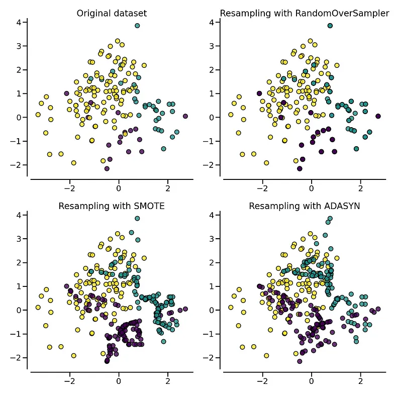
The following plot illustrates the difference between ADASYN and SMOTE. ADASYN will focus on the samples which are difficult to classify with a nearest-neighbors rule while regular SMOTE will not make any distinction. Therefore, the decision function depending of the algorithm.
X, y = create_dataset(n_samples=150, weights=(0.05, 0.25, 0.7))

fig, axs = plt.subplots(nrows=1, ncols=3, figsize=(20, 6))

models = {
    "Without sampler": clf,
    "ADASYN sampler": make_pipeline(ADASYN(random_state=0), clf),
    "SMOTE sampler": make_pipeline(SMOTE(random_state=0), clf),
}

for ax, (title, model) in zip(axs, models.items()):
    model.fit(X, y)
    plot_decision_function(X, y, model, ax=ax, title=title)

fig.suptitle(f"Decision function using a {clf.__class__.__name__}")
fig.tight_layout()
